Convexity

TOC

• Introduction
• Convex set
• Convex function
• Examples
• Derivatives

Introduction

Convexity is an important concept in machine learning, especially in optimization problems. Many optimization algorithms are designed to find the minimum of a convex function because a convex function has only one minimum point, and the minimum point can be found using efficient algorithms. In contrast, non-convex functions may have multiple local minimum points, and it may be difficult to find the global minimum.

In machine learning, convexity is important for many tasks, including linear regression, logistic regression, support vector machines, and neural networks. The loss function used in these tasks is typically convex, which allows efficient optimization using algorithms such as gradient descent.

Convex set

A set C is convex if you connect any two points in that set \(x_1, x_2 \in C\), the line connecting them would lie in the set completely, too. Mathematically, \(\forall 0 \leq \theta \leq 1, x_{\theta} = \theta x_1 + (1 - \theta) x_2 \in C\).

Examples of convex set are hyperplanes and halfspaces. A hyperplane in n-dimensional space is the set of points satisfying the equation: \(a_1 x_1 + a_2 x_2 + ... + a_n x_n = a^T x = b\) with \(b, a_i (i = 1,2,..,n) \in R\). For \(a^T x_1 = a^T x_2 = b\) and \(0 \leq \theta \leq 1: a^T x_{\theta} = a^T (\theta x_1 + (1 - \theta) x_2)) = \theta b + (1 - \theta) b = b\). A halfspace in n-dimensional space is the set of points that satisfies the following inequality: \(a_1 x_1 + a_2 x_2 + ... + a_n x_n = a^T x \leq b\) with \(b, a_i (i = 1,2,..n) \in R\).

Another example is a norm ball. An Euclidean ball is the set of points that satisfies: \(B(x_c, r) = \{x \mid \mid\mid x - x_c \mid\mid_2 \leq r \}\). To prove that this is a convex set, we let any \(x_1, x_2 \in B(x_c, r)\) and \(0 \leq \theta \leq 1\):

\(\mid\mid x_{\theta} - x_c \mid\mid_2 = \mid\mid \theta(x_1 - x_c) + (1-\theta(x_2 - x_c) \mid\mid_2 \leq \theta \mid\mid x_1 - x_c \mid\mid_2 + (1-\theta) \mid\mid x_2 - x_c \mid\mid_2 \leq \theta r + (1-\theta)r = r\). So \(x_{\theta} \in B(x_c, r)\).

Ellipsoids are convex sets, too.

The thing is, if we use norm p (\(p \in R, p >= 1\)): \(\mid\mid x\mid\mid_p = (\mid x_1 \mid^p + ... + \mid x_n \mid^p)^{1/p}\), we end up with convex sets too. Mahalanobis distance is a norm too. Mahalanobis norm of a vector \(x \in R^n\) is: \(\mid\mid x \mid\mid_A = \sqrt{x^T A^{-1} x}\), with A being a matrix such that \(x^T A^{-1} x \geq 0, \forall x \in R^n\).

The intersection of halfspaces and hyperplanes are also convex. The name is a polyhedra. For a halfspace \(a_i^T x \leq b_i, \forall i = 1,2..m\). For a hyperplane \(c_i^T x = d_i, \forall i = 1,2...p\). With \(A = {[a_1, a_2..a_m]}, b={[b_1,b_2..b_m]}^T, C={[c_1,c_2..c_p]}, d={[d_1, d_2...d_p]}^T\) the polyhedra is \(A^T x \leq b, C^T x = d\).

A point is a convex combination of all points \(x_1, x_2, ... x_k\) if \(x = \theta_1 x_1 + \theta_2 x_2 + ... + \theta_k x_k\) with \(\theta_1 + \theta_2 + ... \theta_k = 1\). The convex hull of a set is the collection of all points that are convex combination of that set. The convex hull is a convex set. The convex hull of a convex set is itself. In other words, the convex hull of a set is the smallest convex set that contains all the set. Two sets are linearly separable if their convex hulls don’t intersect. Going further, we are defining the separating hyperplane theorem: if two nonempty convex sets C and D are disjoint (no intersection), then there exists vector a and scalar b such that \(a^T x \leq b, \forall x \in C\) and \(a^T x \geq b, \forall x \in D\). The set of all points x satisfying \(a^T x = b\) is a hyperplane, and it is a separating hyperplane.

Convex function

A function is convex if its domain is a convex set and when we connect any two points on the graph of that function, we have a line above or on the graph. Mathematically, a function \(f: R^n \to R\) is a convex function if domain of f is convex and \(f(\theta x + (1 - \theta) y) \leq \theta f(x) + (1 - \theta) f(y) \forall x,y \in\) domain of f and \(0 \leq \theta \leq 1\)

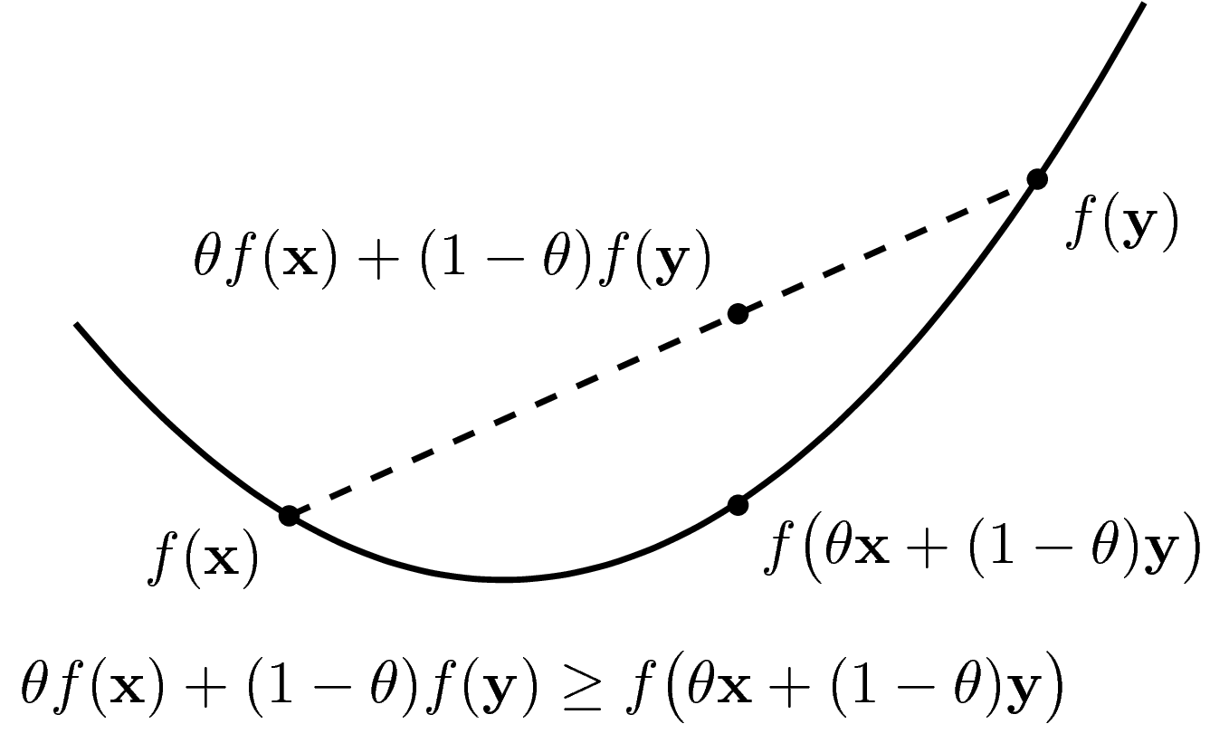Image: graph of a convex function

Similarly, a function \(f: R^n \to R\) is strictly convex if the domain of f is a convex set and \(f(\theta x + (1 - \theta) y) < \theta f(x) + (1 - \theta) f(y), \forall x, y \in\) domain of f and \(x \neq y, 0 < \theta < 1\).

We can do the same for concave and strictly concave functions. If a function is strictly convex and it has a minimum then that minimum is a global minimum. Here are some properties:

• If f(x) is convex then af(x) is convex if a > 0 and concave if a < 0

• The sum of two convex functions is a convex function with the domain to be the intersection of the two functions (the intersection of two convex sets is a convex set)

• If \(f_1, f_2,.. f_m\) is convex then \(f(x) = max \{f_1(x), f_2(x),...f_m(x)\}\) is convex on the domain set being the intersection of all the domain sets.

Examples

Examples of univariate convex functions:

• y = ax + b since the line connecting any two points lie on the graph of it

• \[y = e^{ax}, a \in R\]

• \(y = x^a\) on \(R^+, a \geq 1\) or \(a \leq 0\)

• the negative entropy \(y = x log x, x \in R^+\)

Examples of univariate concave functions:

• y = ax + b since -y is a convex function. Note that y = ax + b is both convex and concave

• \[y = x^a, x \in R^+, 0 \leq a \leq 1\]
• \[y = log(x)\]

\(f(x) = a^T x + b\) is called an affine function. It can be written in matrix form: \(f(X) = tr(A^T X) + b\). The quaratic function \(f(x) = ax^2 + bx + c\) is convex if a > 0, concave if a < 0. It can also be written in matrix form with vector \(x = {[x_1, x_2,...x_n]}: f(x) = x^T A x + b^T x + c\). Usually A is a symmetric matrix (\(a_{ij} = a_{ji} \forall i,y\)). If A is positive semidefinite, the f(x) is a convex function. If A is negative semidefinite (\(x^T A x \leq 0 \forall x\)), f(x) is a concave function.

Derivatives

For differential function, we can check the derivatives to see whether it is convex or not. The definition of the tangient of function f at a point \((x_0, f(x_0)) : y = f'(x_0) (x - x_0) + f(x_0)\). For multivariate function, let \(\nabla f(x_0)\) to be the gradient of function f at point \(x_0\), the tangient surface is: \(y = \nabla f(x_0)^T (x - x_0) + f(x_0)\). We have the condition for f to be convex, with the convex domain, and differential everywhere: if and only if \(\forall x, f(x) \geq f(x_0) + \nabla f(x_0)^T(x-x_0)\). Similar, a function is strictly convex if the equality only happens at \(x = x_0\). Visually, a function is convex if the tangient at any point of the graph lies below the graph.

For multivariate function, i.e. the variable is a vector of dimension d. Its first derivative is a vector of d dimensions. The second derivative is a square matrix of d x d. The second derivative is denoted \(\nabla^2 f(x)\). It is also called the Hessian. A function having the second order derivative is convex if the domain is convex and its Hessian is a semidefinite positive matrix for all x in the domain: \(\nabla^2 f(x) \geq 0\). If Hessian is a positive definite matrix then the function is strictly convex. Similarly, if the Hessian is a negative definite then the function is strictly concave. For univariate functions, this condition means \(f''(x) \geq 0 \forall x \in\) the convex domain.

We have some examples:

• The negative entropy function \(f(x) = x log(x)\) is strictly convex since the domain x > 0 is convex and \(f''(x) = \frac{1}{x}\) is greater than 0 with all x in the domain.

• \(f(x) = x^2 + 5 sin(x)\) is not a convex function since the second derivative \(f''(x) = 2 - 5 sin(x)\) can have a negative value.

• The cross entropy function is a strictly convex function. For two probabilities x and 1 - x, 0 < x < 1, a is a constant in [0,1]: f(x) = -(alog(x) + (1-a)log(1-x)) has the second derivative to be \(\frac{a}{x^2} + \frac{1-a}{(1-x)^2}\) is a positive number.

• If A is a positive definite matrix \(f(x) = \frac{1}{2} x^T A x\) is convex since its Hessian is A - a positive definite matrix.

• For negative entropy function with two variables f(x,y) = x log(x) + y log(y) on the positive set of x and y. This function has the first derivative to be \({[log(x) + 1, log(y) + 1]}^T\) and its Hessian to be:

\[\begin{bmatrix} 1/x & 0 \\ 0 & 1/y \\ \end{bmatrix}\]

This is a diagonal matrix with the positive entries so it is a positive definite matrix. Therefore the negative entropy is a strictly convex funciton.

Jensen’s Inequality

Given a convex function f, we have the generalization of the convexity definition:

\[\sum_{i} \alpha_i f(x_i) \geq f(\sum_i \alpha_i x_i)\]

and \(E_X {[f(X)]} \geq f(E_X{[X]})\) where \(\sum_i \alpha_i = 1\) and \(\alpha_i \geq 0\), X is a random variable. In other words, the expectation of a convex function is no less than the convex function of expectation.

Properties

Local Minima are Global Minima

Consider a convex function f on a convex set X. Suppose that \(x^* \in X\) is a local minimum. So that there exists a small positive value p for \(x \in X\) that satisfies \(0 < \mid x - x^* \mid \leq p\) then \(f(x^*) < f(x)\). To prove that this is also the global minimum, we use contradiction. Assume that \(x^*\) is not the global minimum: there exists \(x' \in X\) so that \(f(x') < f(x^*)\). This means that there exists \(\lambda \in [0,1), \lambda = 1 - \frac{p}{\mid x^* - x' \mid}: 0 < \mid \lambda x^* + (1 - \lambda) x' - x^* \mid \leq p\).

However, according to the definition of convex function, we have:

\(f(\lambda x^* + (1 - \lambda) x' \leq \lambda f(x^*) + (1 - \lambda) f(x')\) \(< \lambda f(x^*) + (1 - \lambda) f(x^*) = f(x^*)\)

This contradicts \(x^*\) being a local minimum. So the global minimum status is proved.