Collaborative Filtering
TOC
Introduction
Collaborative filtering is a technique that is mainly used in recommendation system to suggest user’s preferences by collecting data from a similar group of users. It assumes that if those people have similar preference and decisions in the past, so will they in the near future. So the prediction can be used as recommendation for the user on the products. Use case: Amazon develops item-to-item collaborative filtering in their recommendation system.
Memory based
The memory based technique is to find users or items similar to the current user in the database and calculate the new rating based in the ratings of similar users or items found.
User based
Let’s start with a user-item rating matrix. We have the colums to be users and rows to be items. For large companies such as Netflix, Amazon, etc, the matrix can be quite large with millions of users and items. And the preference of a user over items can be obtained implicitly such as when a user watch a movie, it is assumed that she likes it. Or when she visits the item multiple times and for long, it can also be graded that she likes it. One issue with this utility matrix is that the company might not be able to obtain all ratings to fill in this matrix since each user might rate a few items only. So the matrix is quite sparse. There are several options to fill in those missing values. First is to place 0 for all the missing values. This is not a good choice since 0 means the lowest rating possible. A better option is to replace N/A with the average. For example, if the lowest is 0 and highest possible is 5, we can use 2.5. However, this has some issue with different kind of users. For example, an easy reviewer might rate 5 stars for a likeable move and for movies she doesn’t like, she rate 3. If we replace her N/A with 2.5, all those movies mean bad movies for her. But for a difficult reviewer, she might only give 3 stars for movies she really likes and 1 star for movies she doesn’t like. If we replace all her N/A with 2.5, we are assuming that she likes all the rest. A more reasonale option is to use a different average which is the average of all the ratings she has done. This alleviates the problem of easy and difficult user mentioned above. After filling those numbers in, we can normalize the matrix by substrating each user’s rating column by their own average. This effectively set all the missing values to 0. Then 0 would be the neutral value and a positive value would mean that that user likes that movie. Likewise, a negative value means that the user doesn’t like that movie. Doing that would make the matrix being stored more efficiently. And since sparse matrices can fit better into memory, it is also better for when we do the calculation.
The next step is to calculate similarity. We can use Euclidean distance or cosine similarity method.
Euclidean distance
The Euclidean distance between two points in the Euclidean space is the length of the line segment between the two. It is also called the Euclidean norm of the two vector difference:
\[d(x,y) = \mid\mid p - q \mid\mid = \sqrt{(p_1 - q_1)^2 + (p_2 - q_2)^2}\]
Image: Euclidean distance between two datapoints
import numpy as np

p1 = np.array([0,1,5,3,2,4])
p2 = np.array([1,3,5,4,1,2])

distance = np.linalg.norm(p1 - p2)
print(distance)
3.3166247903554
Cosine similarity
Cosine similarity method is to calculate the cosine of the angle between two vectors formed by the two datapoints: \(cos(u_1, u_2) = \frac{u_1^T u_2}{\mid \mid u_1 \mid\mid_2 . \mid\mid u_2\mid\mid_2}\). With \(u_1, u_2\) being normalized vectors. The value of the similarity would conveniently be between -1 and 1. A value of 1 means perfectly similar (the angle between these two vectors is 0). A value of -1 means perfectly dissimilar (the two vectors are on opposite directions). This means that when the behavior of the two users are opposite, they are not similar.
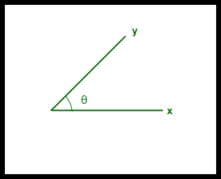
Image: the angle between two vector formed by two datapoints
import numpy as np

def cosine_similarity(A, B):
    dot_product = np.dot(A, B)
    norm_a = np.linalg.norm(A)
    norm_b = np.linalg.norm(B)
    return dot_product / (norm_a * norm_b)

# example vectors
p1 = np.array([0,1,5,3,2,4])
p2 = np.array([1,3,5,4,1,2])

print(cosine_similarity(p1, p2))
0.900937462695559
Other similarity indices that can be used are Pearson correlation coefficient, Jaccard similarity, Spearman rank correlation and mean squared difference. The Pearson correlation coefficient is the linear relation between the two samples. It is the covariance of the two variables divided by the multiplication of the two standard deviations: \(\rho_{X,Y} = \frac{cov(X,Y)}{\sigma_X \sigma_Y}\). Spearman rank correlation is the Pearson correlation equation but for rank variables. Jaccard similarity is when we count the number of items in the intersection set of the two sets then divide it by the number of items in the union set of the two sets: \(J(X,Y) = \frac{\mid A \cap B \mid}{\mid A \cup B \mid}\). Mean squared difference is a popular measure for the distance between points.
def jaccard_similarity(setA, setB):
    intersection = len(setA & setB)
    union = len(setA | setB)
    return intersection / union

# example sets
p1 = np.array([0,1,5,3,2,4])
p2 = np.array([1,3,5,4,1,2])

print(jaccard_similarity(p1,p2))
1.0
Notice that the two vectors have the same ratings but in different order. In this case, the jaccard similarity shows the perfect similarity which is not reasonable. If you plan to try this similarity index, please do keep this in mind.
from scipy.stats import spearmanr

# Example data
p1 = np.array([0,1,5,3,2,4])
p2 = np.array([1,3,5,4,1,2])

correlation, p_value = spearmanr(p1, p2)

print("Spearman Rank Correlation: ", correlation)
Spearman Rank Correlation: 0.6667366910003157
After establishing a way to calculate similarity, we then can move on to predict the rating. To calculate the rating prediction of user U for item I: we choose a list of top 5-10 most similar users who already rated I, then we take average of those ratings: \(R_U = \frac{\sum_{u=1}^n R_u}{n}\). This equation takes all the top similar users equally. Another choice is that we can weigh them accordingly: \(R_U = \frac{\sum_{u=1}^n R_u * W_u}{\sum_{u=1}^n W_u}\). The weights can be the similarity index for each user. Overall, this method is like asking your friends’ suggestion when you want to see a new movie. We know that our friends have similar taste to us and so we can trust them. Their recommendations would be a reliable source of information.
Code example
In this example, with the same movie lens dataset, we are going to do collaborative filtering: we create a user-item matrix (the utility matrix). Then we substract each rating with the average of rating of that user (this technique is to center the ratings). Then we fill N/A with 0. The next step is to calculate the cosine similarity for all users. By doing this, the system can list out the most similar users for a given user. Then if we need rating for a movie, we calculate the weighted average of the ratings by those most similar users.
import pandas as pd
ratings = pd.read_csv('ml-latest-small/ratings.csv', low_memory=False)
ratings.head()
| userId | movieId | rating | timestamp | |
|---|---|---|---|---|
| 0 | 1 | 1 | 4.0 | 964982703 |
| 1 | 1 | 3 | 4.0 | 964981247 |
| 2 | 1 | 6 | 4.0 | 964982224 |
| 3 | 1 | 47 | 5.0 | 964983815 |
| 4 | 1 | 50 | 5.0 | 964982931 |
user_movie_matrix = ratings.pivot(index='userId', columns='movieId', values='rating')
user_movie_matrix = user_movie_matrix.apply(lambda row: row - row.mean(), axis=1)
user_movie_matrix.fillna(0, inplace=True)
user_movie_matrix.head()
| movieId | 1 | 2 | 3 | 4 | 5 | 6 | 7 | 8 | 9 | 10 | ... | 193565 | 193567 | 193571 | 193573 | 193579 | 193581 | 193583 | 193585 | 193587 | 193609 |
|---|---|---|---|---|---|---|---|---|---|---|---|---|---|---|---|---|---|---|---|---|---|
| userId | |||||||||||||||||||||
| 1 | -0.366379 | 0.0 | -0.366379 | 0.0 | 0.0 | -0.366379 | 0.0 | 0.0 | 0.0 | 0.0 | ... | 0.0 | 0.0 | 0.0 | 0.0 | 0.0 | 0.0 | 0.0 | 0.0 | 0.0 | 0.0 |
| 2 | 0.000000 | 0.0 | 0.000000 | 0.0 | 0.0 | 0.000000 | 0.0 | 0.0 | 0.0 | 0.0 | ... | 0.0 | 0.0 | 0.0 | 0.0 | 0.0 | 0.0 | 0.0 | 0.0 | 0.0 | 0.0 |
| 3 | 0.000000 | 0.0 | 0.000000 | 0.0 | 0.0 | 0.000000 | 0.0 | 0.0 | 0.0 | 0.0 | ... | 0.0 | 0.0 | 0.0 | 0.0 | 0.0 | 0.0 | 0.0 | 0.0 | 0.0 | 0.0 |
| 4 | 0.000000 | 0.0 | 0.000000 | 0.0 | 0.0 | 0.000000 | 0.0 | 0.0 | 0.0 | 0.0 | ... | 0.0 | 0.0 | 0.0 | 0.0 | 0.0 | 0.0 | 0.0 | 0.0 | 0.0 | 0.0 |
| 5 | 0.363636 | 0.0 | 0.000000 | 0.0 | 0.0 | 0.000000 | 0.0 | 0.0 | 0.0 | 0.0 | ... | 0.0 | 0.0 | 0.0 | 0.0 | 0.0 | 0.0 | 0.0 | 0.0 | 0.0 | 0.0 |
5 rows × 9724 columns
from sklearn.metrics.pairwise import cosine_similarity
cosine_sim = cosine_similarity(user_movie_matrix, user_movie_matrix)
user_similarity_df = pd.DataFrame(cosine_sim)
user_similarity_df
| 0 | 1 | 2 | 3 | 4 | 5 | 6 | 7 | 8 | 9 | ... | 600 | 601 | 602 | 603 | 604 | 605 | 606 | 607 | 608 | 609 | |
|---|---|---|---|---|---|---|---|---|---|---|---|---|---|---|---|---|---|---|---|---|---|
| 0 | 1.000000 | 0.001265 | 0.000553 | 0.048419 | 0.021847 | -0.045497 | -0.006200 | 0.047013 | 0.019510 | -0.008754 | ... | 0.018127 | -0.017172 | -0.015221 | -0.037059 | -0.029121 | 0.012016 | 0.055261 | 0.075224 | -0.025713 | 0.010932 |
| 1 | 0.001265 | 1.000000 | 0.000000 | -0.017164 | 0.021796 | -0.021051 | -0.011114 | -0.048085 | 0.000000 | 0.003012 | ... | -0.050551 | -0.031581 | -0.001688 | 0.000000 | 0.000000 | 0.006226 | -0.020504 | -0.006001 | -0.060091 | 0.024999 |
| 2 | 0.000553 | 0.000000 | 1.000000 | -0.011260 | -0.031539 | 0.004800 | 0.000000 | -0.032471 | 0.000000 | 0.000000 | ... | -0.004904 | -0.016117 | 0.017749 | 0.000000 | -0.001431 | -0.037289 | -0.007789 | -0.013001 | 0.000000 | 0.019550 |
| 3 | 0.048419 | -0.017164 | -0.011260 | 1.000000 | -0.029620 | 0.013956 | 0.058091 | 0.002065 | -0.005874 | 0.051590 | ... | -0.037687 | 0.063122 | 0.027640 | -0.013782 | 0.040037 | 0.020590 | 0.014628 | -0.037569 | -0.017884 | -0.000995 |
| 4 | 0.021847 | 0.021796 | -0.031539 | -0.029620 | 1.000000 | 0.009111 | 0.010117 | -0.012284 | 0.000000 | -0.033165 | ... | 0.015964 | 0.012427 | 0.027076 | 0.012461 | -0.036272 | 0.026319 | 0.031896 | -0.001751 | 0.093829 | -0.000278 |
| ... | ... | ... | ... | ... | ... | ... | ... | ... | ... | ... | ... | ... | ... | ... | ... | ... | ... | ... | ... | ... | ... |
| 605 | 0.012016 | 0.006226 | -0.037289 | 0.020590 | 0.026319 | -0.009137 | 0.028326 | 0.022277 | 0.031633 | -0.039946 | ... | 0.053683 | 0.016384 | 0.098011 | 0.061078 | 0.019678 | 1.000000 | 0.017927 | 0.056676 | 0.038422 | 0.075464 |
| 606 | 0.055261 | -0.020504 | -0.007789 | 0.014628 | 0.031896 | 0.045501 | 0.030981 | 0.048822 | -0.012161 | -0.017656 | ... | 0.049059 | 0.038197 | 0.049317 | 0.002355 | -0.029381 | 0.017927 | 1.000000 | 0.044514 | 0.019049 | 0.021860 |
| 607 | 0.075224 | -0.006001 | -0.013001 | -0.037569 | -0.001751 | 0.021727 | 0.028414 | 0.071759 | 0.032783 | -0.052000 | ... | 0.069198 | 0.051388 | 0.012801 | 0.006319 | -0.007978 | 0.056676 | 0.044514 | 1.000000 | 0.050714 | 0.054454 |
| 608 | -0.025713 | -0.060091 | 0.000000 | -0.017884 | 0.093829 | 0.053017 | 0.008754 | 0.077180 | 0.000000 | -0.040090 | ... | 0.043465 | 0.062400 | 0.015334 | 0.094038 | -0.054722 | 0.038422 | 0.019049 | 0.050714 | 1.000000 | -0.012471 |
| 609 | 0.010932 | 0.024999 | 0.019550 | -0.000995 | -0.000278 | 0.009603 | 0.068430 | 0.017144 | 0.051898 | -0.026004 | ... | 0.021603 | 0.030061 | 0.051255 | 0.015621 | 0.069837 | 0.075464 | 0.021860 | 0.054454 | -0.012471 | 1.000000 |
610 rows × 610 columns
def most_similar_users(user_id, user_similarity_df, n=5):
    # Get the series of similarity scores for the given user
    user_similarity_series = user_similarity_df.loc[user_id]

    # Exclude the user's own id (a user is always most similar to themselves)
    user_similarity_series = user_similarity_series.drop([user_id])

    # Get the most similar users
    most_similar_users = user_similarity_series.nlargest(n)

    return most_similar_users

# Get the 5 users most similar to user 1

similar_users = most_similar_users(1, user_similarity_df)
print(similar_users)
188    0.134677
245    0.106334
377    0.099583
208    0.089539
226    0.085428
Name: 1, dtype: float64
Notice that 0.13 doesn’t show really high similarity.
def get_ratings_for_movie(movie_id, similar_users, ratings_df):
    # Get the ratings of the most similar users for the given movie
    ratings = user_movie_matrix.loc[similar_users.index, movie_id]

    return ratings

# Get their ratings for the target movie
new_ratings = get_ratings_for_movie(2, similar_users, ratings)

print(new_ratings)
188    0.000000
245    0.000000
377    0.000000
208    0.000000
226   -0.476331
Name: 2, dtype: float64
import numpy as np
np.dot(similar_users, new_ratings)
-0.04069219402243481
User 1 is not likely to like movie 2. Or we can say that she/he is likely to be neutral. Since 4 out of the most 5 similar users (her neighbours) hasn’t watched the movie yet.
Item based
In the case of user based rating matrix, the matrix is usually sparse since each user only rates a few products. When one user changes rating or rate more, the average rating of that user changes and the normalization needs to be redone, leading to the need to redo the rating matrix as well. An approach that Amazon proposes, is to calculate the similarity among items then we can predict the rating of a new item based on those already rated items of the same user. Usually, the number of items are smaller than the number of users. This makes similarity matrix smaller and easier for calculation. Pick out a list of top 5-10 most similar items to the current one, rated by the user. Take their average or weighted average to indicate its rating. This method is developed by Amazon and can be used when there are more users than items, since it is more stable and faster. It is not very suited for datasets with browsing or entertainment related items.
Model based
First to reduce the large but sparse user item matrix by matrix factorization. Matrix factorization is to breaking down a large matrix into a product of smaller ones. A = X * Y. For example a matrix of m users * n items can be factorized into the product of user matrix X (m * p feature)s and item matrix Y (p * n features). P are called latent features which means they are hidden characteristics of the user and the items.
If we reduce the dimension p into k < p, though, we force the algorithm to choose k main hidden characteristics that describe the most of the data possible. Then we multiple X_k (m * k) with Y_K (k * n), we get a new A’ that approximates the original A. But in this new A’, the missing values are filled in. This is how recommendation system works (similar to PCA). A general idea of this technique is called bottlenecking, we bottleneck the model so that only principal information comes through. And we end up with the “true” pattern underlying the dataset.
SVD
One of the popular algorithm to factorize matrix into meaningful components is the singular value decomposition algorithm. This method was introduced at length in a previous post on LSD/LSA (laten semantic analysis) for document processing. It is to factorized the utility matrix into a multiplication of user and item matrix: \(A = U \Sigma V^T\)
where U and V are orthogonal matrices, \(\Sigma\) being the diagonal matrix containing the singular values of A. The singular values in \(\Sigma\) are sorted in decreasing order and the number of non zero singular values indicates the rank of matrix A.
from scipy.sparse.linalg import svds
import numpy as np
np.set_printoptions(suppress=True)

# A simple user-item matrix
A = np.array([
    [0,1,5,3,4,5],
    [1,3,5,4,0,3],
    [3,4,2,0,2,1],
    [2,2,1,0,2,3]
])

# Perform SVD
U, s, VT = np.linalg.svd(A)

# print("U:\n", U)
# print("S:\n", S)
# print("VT:\n", VT)

# Construct diagonal matrix in SVD
S = np.zeros(A.shape)
for i in range(min(A.shape)):
    S[i, i] = s[i]

# Reconstruct Original Matrix
A_reconstructed = np.dot(U, np.dot(S, VT))
print("A (Full SVD):\n", A_reconstructed)

# Perform Truncated SVD
k = 2  # number of singular values to keep

U_k = U[:, :k]
S_k = S[:k, :k]
VT_k = VT[:k, :]

# Reconstruct Matrix using Truncated SVD
A_approx = np.dot(U_k, np.dot(S_k, VT_k))
print("A' (Truncated SVD):\n", A_approx.round(2))
A (Full SVD):
 [[0. 1. 5. 3. 4. 5.]
 [1. 3. 5. 4. 0. 3.]
 [3. 4. 2. 0. 2. 1.]
 [2. 2. 1. 0. 2. 3.]]
A' (Truncated SVD):
 [[ 0.23  1.69  5.33  3.77  2.38  4.56]
 [ 0.73  2.    4.42  2.9   2.19  3.83]
 [ 3.11  3.84  1.62 -0.11  1.9   1.64]
 [ 1.9   2.56  1.8   0.52  1.51  1.69]]
PCA
PCA also decomposes the matrix into smaller matrices (in this case with eigenvectors). PCA algorithm has been introduced in a previous post.
from sklearn.decomposition import PCA
from sklearn.preprocessing import StandardScaler
import numpy as np

# Assuming you have a dataset X with n samples and m features
X = np.array([
    [0,1,5,3,2,4],
    [1,3,5,4,1,2],
    [3,4,2,0,0,1],
    [2,2,1,0,2,3]
])
# Standardize the features
X = StandardScaler().fit_transform(X)

# Create a PCA object
pca = PCA(n_components=2) # we are reducing the dimension to 2

# Fit and transform the data
X_pca = pca.fit_transform(X)

print("original shape:   ", X.shape)
print("transformed shape:", X_pca.shape)
original shape:    (4, 6)
transformed shape: (4, 2)
NMF
Non negative matrix factorization is a technique that decomposes a non negative matrix into the product of two non negative matrices: \(V \approx W * H\) with the constraint that V,W,and H does not contain any negative elements. The factorization is performed using an iterative optimization algorithm that minimizes the difference between V and the product of W and H: \(\mid\mid V - WH \mid\mid^2 = \sum (V - WH)^2\). After having the two smaller matrices, we can predict the missing values using matrix multiplication.
from sklearn.decomposition import NMF
import numpy as np

# Create a simple matrix
V = np.array([
    [0,1,5,3,2,4],
    [1,3,5,4,1,2],
    [3,4,2,0,0,1],
    [2,2,1,0,2,3]
])
# Create an NMF instance
nmf = NMF(n_components=2, init='random', random_state=0)

# Fit the model
W = nmf.fit_transform(V)
H = nmf.components_

print("W:\n", W)
print("H:\n", H.round(2))
print("Reconstruction:\n", np.dot(W, H).round(2))
W:
 [[1.53156606 0.        ]
 [1.29777613 0.68617373]
 [0.         2.01368557]
 [0.25974709 1.23548283]]
H:
 [[0.   0.89 3.29 2.39 1.1  2.1 ]
 [1.52 1.9  0.78 0.   0.3  0.75]]
Reconstruction:
 [[0.   1.36 5.03 3.66 1.69 3.21]
 [1.04 2.46 4.8  3.1  1.64 3.24]
 [3.06 3.83 1.57 0.   0.61 1.51]
 [1.88 2.58 1.82 0.62 0.66 1.47]]
Hybrid
A hybrid model is one that makes use of both methods (memory based and model based). This is to leverage the strengths and compensate for weaknesses of both methods. For example, a hybrid model might use the model based method to predict a rating for an item, and then use a memory based method to generate prediction from similar users or items. So that they can compare or combine those predictions in some ways. The hybrid model clearly enjoys the patterns learned by the model based method, at the same time can keep the personalization by the memory method.
Deep learning
Auto encoder
An auto encoder would learn the internal structure of a dataset, with hidden features, and then make prediction when new datapoint come in. Since a neural network approximates a function, this function also does bottleneck: to force the data in some way so that only the most important information can come through. Then the resulting model can be used to predict the missing values. Auto encoder has been introduced at length in a previous post.